Converter simulator

Pick a topology or a preset, choose the load, and set the parameters in SI units, with or without a prefix (100u and 0.0001 are the same inductance, 200k and 200000 the same frequency): type a value, or drag its slider, which spans one decade either side of the value (0 to 1 for the duty ratio). A field that does not hold a number turns red. A new load, or the source switched on, fills each field it adds with an example’s value, which you can then change. The simulator computes one period of the periodic steady state and shows:

the waveforms: inductor current and voltage, diode current, switch voltage and output voltage, and the battery’s current when there is one;
the conduction mode it detects, with $K$ and $K_\mathrm{crit}$ ;
the simulated values next to the catalogue’s equations at the same operating point;
the losses and the efficiency computed from the waveforms, and where the load’s power goes.

When the circuit has no periodic steady state, it says why and shows the start-up from rest instead (below).

Everything runs in your browser on the pe-core engine that the test suite validates. The URL holds the whole state, and the “Try it” links on the learning pages open the simulator with a preset.

What is modelled

Each converter is a set of linear circuits, one for each interval of the switching period: switch on, switch off with the diode conducting, and, in DCM, the idle interval [Erickson & Maksimović 2020, Ch. 2], [Erickson & Maksimović 2020, Ch. 5].

Switches and diodes. The transistor is an ideal switch with an optional on-resistance and an ideal body diode across it. The diode is a constant forward drop that blocks ideally, with no reverse recovery. The inductor can have a winding resistance. A current that would reverse through a diode stops instead: the forward converter’s rectifier blocks while its output is above $n V_g$ less the diode drop. A negative current through the switch flows through its body diode, which conducts at zero volts: after turn-off until the current reaches zero, and while the switch is on too, when the diode takes the current from the on-resistance.
Transformers. They are ideal (1:n with $n$ the secondary turns over the primary turns) except for the magnetizing inductance. There is no leakage inductance.
Transitions. Without a capacitance across the switch they are instantaneous. With one, the inductor current charges it after turn-off until the diode takes over. While the diode conducts, the capacitance follows the switch voltage, which moves with the output and input ripple, so it takes its share of their capacitors’ current. Once the diode current reaches zero, the inductance rings with the capacitance (ringing frequency). The switch’s body diode clamps the ringing at zero switch voltage, and the energy in the capacitance is lost at every turn-on (capacitive turn-on loss). The input energy therefore equals the output energy plus the losses, also with the capacitance.
Source-driven mode. The input can be a Thevenin source charging a bus capacitor instead of a fixed voltage. With a fixed output and a fixed duty ratio, this reproduces the constant-voltage sink of the flyback (the pinned input voltage).

Loads

The output capacitor $C$ has across it one of:

a resistor $R$ ;
a battery: its open-circuit voltage $V_b$ behind its internal resistance $R_b$ , the Rint model [He et al. 2011, Sec. 2.1];
a battery and a resistor;
nothing, so that the capacitor charges from its start voltage $V_0$ .

Or the output is an ideal fixed voltage $V$ (a stiff battery or a regulated bus), with no capacitor. The battery’s current is

I_b = \frac{V - V_b}{R_b}

$I_b$: battery current (charging positive)
$R_b$: battery internal resistance
$V$: output voltage
$V_b$: battery open-circuit voltage

Battery current in the Rint model✓ verified by 8 tests

Assumptions, convention and source

Assumptions

battery modelled as its open-circuit voltage behind an internal resistance (Rint model)

Notes

the battery charges when its terminals are above its open-circuit voltage and discharges below it; the open-circuit voltage and the resistance depend on the state of charge, the state of health and the temperature, which the simulator holds constant over the periods it computes

Source

He et al. 2011, Sec. 2.1 (The Rint Model)

Equation id

bat.rint · equations.yaml entry

It is positive while the battery charges. In a real battery the resistance and the open-circuit voltage depend on the state of charge, the state of health and the temperature [He et al. 2011, Sec. 2.1]; the simulator holds both constant: a battery at one state of charge. Over the periods it computes (a handful to find a steady state, a few hundred at most for a start-up) the charge a battery takes is a tiny part of any real battery’s capacity. The load table below the charts splits the battery’s power into what its open-circuit voltage takes ( $V_b$ times the battery’s average current) and what its internal resistance dissipates ( $R_b$ times the mean square of that current).

When there is no steady state

A periodic steady state needs every state to return to its start at the end of the period. For an inductor this is the volt-second balance (volt-second balance), for a capacitor the charge balance (charge balance) [Erickson & Maksimović 2020, Ch. 2]. Some circuits cannot meet them, and the simulator then says which state keeps changing, by how much per cycle, and shows the start-up from rest (no current, the capacitor at its start voltage or the battery’s) in place of the steady-state period:

An inductor current that runs away. A fixed output fed in CCM from a fixed input balances the inductor’s volt-seconds at one duty ratio only. Above it, the average voltage the inductance sees over a cycle is positive, and the current grows by the same amount every cycle (change over one period). Below it, the current falls to zero within the cycle instead, and the converter settles in DCM. The message gives the change per cycle, that average voltage, and the duty ratio that would balance with ideal parts: the catalogue’s CCM conversion ratio solved for $D$ , with the fixed output over the input as the ratio (negative for the buck-boost, whose output is inverted). A flyback into a fixed output, for example, gains in each on-interval the rise that its magnetizing current has from zero in DCM (the on-interval's rise), and loses in the off-interval only what the output voltage, reflected to the primary, takes away in the time left. The forward converter’s magnetizing current walks up in the same way above its reset limit (maximum duty ratio), which the message then names. At exactly the balancing duty ratio, with ideal parts, the volt-seconds balance whatever the current: every current that starts and ends a period at the same value is a steady state, and the simulator reports the one it reaches from its starting point. A duty ratio so close to it that the current’s change per cycle is less than a millionth of how far it moves within the period passes the convergence test below, and counts as balanced.
A capacitor that charges without bound. With nothing across it, the output capacitor keeps what every cycle delivers. Behind a boost, buck-boost or flyback without a capacitance across the switch, every cycle stores energy in the inductance and hands it on whatever the output’s voltage, so the capacitor charges without bound. The message gives the voltage reached and the gain per cycle.
Anything else that has not settled within the cycle limit, such as an undamped L-C ringing.

A capacitor alone does settle behind the other converters:

Behind a buck it settles at the input’s voltage, from below or from above, because the switch conducts both ways. The search starts there.
Behind a forward converter, and behind a boost, buck-boost or flyback with a capacitance across the switch, it stops once no more charge reaches it: for the forward converter at about $n V_g$ less the diode drop (a little below it with $R_\mathrm{on}$ ) or above, since its rectifier lets no current back; for the others at the voltage to which the inductance can no longer lift the node capacitance. Every voltage above that one is a steady state too, and which one the capacitor keeps depends on its start-up: an L-C charge can overshoot and keep its peak, the first periods from rest can carry more energy than the periodic ringing, and an input bus that sags and recovers moves the voltage on the way. So the simulator follows the start-up from $V_0$ and searches from where the capacitor stops charging: no charge for 50 periods in a row, or for 3 with every other state repeating itself. A start-up that charges again after such a pause ends above the voltage reported. Where the charge per period instead shrinks steadily towards a limit, with every other state repeating itself, it searches for that limit, the lowest voltage that no charge reaches; the start-up, charging in ever smaller steps, stops just above it (by about a hundred-millionth of the voltage in the cases tried). It follows at most 4000 periods and two million sub-steps: with a node capacitance, whose ringing needs more sub-steps, that is 100 to 1000 periods, and random trials often reach it. A start-up still charging then is searched from where it got to; if that search fails, or finds a voltage below the one the start-up reached, the steady state is found from above instead, with the capacitor high enough that no charge reaches it, and the voltage brought down to the lowest one that no charge reaches. Such a start-up is reported below the voltage it would stop at, by up to about 0.07 % in random trials, and a steady state found from above can lie a few millionths above it. The periods followed count in the number of cycles the result reports.

Without a steady state there is no conduction mode, no comparison with the equations and no table of the load or the losses: each of them describes a periodic steady state.

Operating modes

Below the charts the steady-state period is split into its modes: each mode is a stretch of the period in which one linear circuit holds (the switch on, the diode conducting, the idle interval of DCM [Erickson & Maksimović 2020, Ch. 5], the node capacitance’s rise and ringing, the forward converter’s reset). Pick a mode with its button, or click on the charts; the charts shade it. For the selected mode the view shows:

the circuit, with the branches that carry current in the mode in colour and the others grey, and an arrow on each coloured branch in the direction its current flows (two heads when the current reverses within the mode). The switch is drawn closed while its gate is on; its body diode, across it, is coloured when it carries the current. Next to each element are its name and its state;
what happens: first which parts conduct in the mode and how they connect; then, for each inductor that carries current, the average voltage across it in the mode, the number in the table (with a winding resistance, split into the drop across the resistance and the voltage across the inductance itself), and what its current does; for the forward converter’s magnetizing inductance, whether its current has returned to zero, the core’s reset, or has not when the switch turns on again; then one sentence each for the output capacitor, the battery or the fixed output, the input or the source and its bus capacitor, from their states in the table;
a table of every element’s state, its current at the start and the end of the mode with its average over it (like the period’s averages, the exact integral over the mode divided by the mode’s length; the voltages’ averages too), and its voltage where the simulator has it. Each current is positive in the direction of the element’s arrow on the circuit, the direction of its average current in the mode; a negative value flows against the arrow. An inductor’s voltage is taken along its arrow too, so that a positive voltage across the inductance goes with a current that grows along the arrow; it includes the drop across the winding resistance. Every other voltage keeps the element’s own direction.

The states are read from the simulated waveforms of the mode, never assumed: an inductor stores energy while its current’s magnitude grows and releases it while it shrinks, and a current that grows and then shrinks within the mode (or the other way round) is reported so; a capacitor or a battery charges while its current flows into its positive terminal; a source delivers while its current leaves its positive terminal, and a source or a fixed output whose current changes direction within the mode carries power both ways; a current that changes sign once is reported with the instant it reverses. The parts that conduct also name the mode: a forward converter’s switch-on interval whose rectifier carries no current that counts is the rectifier blocked, and a switch-off interval whose diode carries none is idle, or ringing with a node capacitance. Each state is read at the samples the simulator records in the mode, every sub-step (a two-thousandth of the period) and both sides of every event: a mode shorter than a sub-step, such as a node capacitance’s rise of a few nanoseconds, is read from its two ends. An inductor’s state also reads its current’s exact extremes in the mode, between the samples: a current that peaks inside the first sub-step after a node capacitance’s rise stores, then releases.

A current smaller than a thousandth of its scale counts as none, in the drawing, the states and the table. The scale is the largest current, during the mode, among the elements the current flows with: the switching cell (the switch, the diodes, the windings, the inductances, the node capacitance and a direct input; a transformer’s primary side and its secondary side apart, since the turns ratio scales one against the other), the output capacitor with the load, the bus capacitor with the source. So the microamperes a node capacitance draws through the input while the diode carries amperes are not a current path, while a ringing that turns the diode on again for a few nanoseconds conducts a current that is that mode’s whole story, however small beside the period’s peak. An inductor’s scale is at most its own largest current over the period: a forward converter’s magnetizing current, a thousandth of the load current, is its own story. A capacitor’s scale is at least what the load or the source draws: a capacitor that alone feeds a megohm resistor counts, one that trickles nanoamperes into a battery drawing amperes does not. The resistor, the battery, a fixed output, and the source with its resistance, which conduct in every mode by nature, are measured against their own largest current over the period. The currents that count at each node must then balance: where they do not (a battery feeding the resistor between its charging pulses, with a current far below a thousandth of theirs), the element at the node with the largest current that does not count is measured against the largest one that does, until every node balances. A wire is coloured when what it passes between the elements on its two sides counts for the smallest-scaled of the elements on either side, so a coloured path never ends at a node. Whether a current that counts grows or shrinks is read more finely, from a millionth of its scale.

Rounding stays below all of this: a current smaller than a billionth of the circuit’s natural current (what its largest voltage builds in one period in its inductance) never counts; a mode shorter than a billionth of the period (a current left at $10^{-21}$ A sends the switch through its body diode for $10^{-26}$ s) joins the mode next to it; and a circuit in which every current is rounding (a capacitor alone at its steady voltage) is shown at rest, without modes and without mode bands on the charts.

The drawing and the table use the same currents, and those come from the model’s outputs for each element: Kirchhoff’s current law holds at every node of the drawn circuit at every instant of the period, for every topology, load, node capacitance and source (sim-schematic.test.ts). Near each mode boundary where a diode’s or an inductor’s current ends, the instant that current last falls through 5 % of its average in the period agrees with ngspice within 3 ns (2.1 ns at worst) in every circuit of the SPICE comparison below.

Under the mode view, All modes at once draws the whole period. First the key waveforms, stacked on one time axis: the gate, the inductor’s current, the switch’s current (its body diode’s included, negative) and the diode’s, the switch’s voltage and the inductor’s voltage; for the forward converter, the magnetizing current and both output diodes’ currents instead of the inductor’s voltage. The boundaries $t_0$ , $t_1$ , … between the modes are dashed, and each row’s largest value stands at its right, with its smallest where there is room. Then comes the circuit of every mode, lettered (a), (b), … in order, with the same colours, arrows and descriptions as the mode view. Like everything on the page, it follows the values in the form. The topology pages show it for their examples, the buck converter’s for one.

How it computes

The ideas below, with worked numbers, are on the page how the in-browser simulator works.

Within an interval the state (inductor current, capacitor voltages) obeys a linear differential equation. The simulator advances it with the exact solution of that equation (a matrix exponential) over sub-steps of one two-thousandth of the switching period, or shorter, so that one period of the circuit’s fastest ring spans at least twenty sub-steps, down to one twenty-thousandth of the period. The fastest ring comes from the eigenvalues of every interval’s equations: the capacitance across the switch, a small output capacitor with the inductance, the input bus. A circuit that rings so fast that a ring would still span fewer than three sub-steps is refused: a diode could turn on and off again between two sub-steps unseen. A start-up drawn without a steady state follows the same rule. The exponential is computed by scaling and squaring with a Padé approximant [Higham 2005], and is formed, and squared, less the identity. Before that, the states are rescaled by powers of two, which is exact, until each state’s couplings to the others are of similar size in both directions (balancing [Parlett & Reinsch 1969]): a tiny bus capacitance behind a source resistance that is not small would otherwise make the matrix far larger than its fastest mode, and the linear solve inside the approximant would then pivot on those large couplings, which costs the slower states their digits. So a time constant far shorter than a sub-step does not cost them.
Events such as the diode current reaching zero or a clamp starting to conduct are located inside a sub-step on the same exact solution, by a search that keeps the event bracketed like bisection (regula falsi in its Illinois variant, which needs far fewer steps). When one event ends a sub-step early, the other conditions are checked again at that instant. A condition that was met earlier in the sub-step, but no longer holds at its end, happened first: for example, a node capacitance’s rise that passes the diode’s turn-on voltage just before its current ends at the peak. The gate edges fall exactly at the start of the period and at the duty ratio.
Averages, powers and extremes. Within an interval every quantity the page reports is a straight (affine) function of the states, and between two samples the states follow the interval’s equations exactly. So the averages, the powers, and the mean squares behind the rms values and the conduction losses are the exact integrals of that solution over every sub-step, not straight lines through the samples. They are taken from the exponential of a larger matrix built from the interval’s equations [Van Loan 1978], rescaled and formed less the identity like the steps, in each state’s deviation from the first state the period visits in that interval, with the rate of change there summed in twice the precision. A quantity whose constant part dwarfs what varies, such as a battery’s current behind a small resistance, then keeps the digits its samples give it: a unit in the last place of the battery’s voltage over its resistance, a resolution that the current of the capacitor beside it shares. A transient faster than a sub-step, such as a time constant far shorter than one, is integrated as exactly as a slow one. Through the same samples, the results agree with a 60-digit integration to a few parts in a trillion of each quantity’s scale in the tested circuits, including ones whose time constant is several hundred billion times shorter than a sub-step, and between two grids of sub-steps to about one part in ten billion. Over hundreds of random circuits, two grids from the same start agree as closely against the circuit’s largest current or voltage, down to the battery current’s resolution, wherever they see the same events; where the currents are themselves only rounding, as in a capacitor alone that has settled, they agree to that rounding. Where one grid sees a diode conduct briefly inside a sub-step and the other does not, they differ by what that conduction carries (see Outside the model below). Each quantity’s largest and smallest value also include a peak between two samples: where its slope changes sign within a sub-step, and where the slope dips through zero and back within one (a ring riding on a steeper ramp). The slope is also checked close to the sub-step’s start, where a fast transient decays. A turn within the rounding of the slope itself is not searched; a quantity that barely moves, at the rounding of its own value, is still searched where its slope turns, which makes a few circuits several times slower. Each slope is the rate of change at the sample, summed in twice the precision and carried along the sub-step like the states, so an input bus behind a tiny source resistance and capacitance, whose slope is what is left of terms many orders of magnitude larger, still has its peak placed to rounding. The plots draw the samples, so a peak narrower than a sub-step can be in the numbers but not in the plot.
Rounding. Within a period the simulator follows each state’s deviation from its value at the start of the period. Its rounding errors then scale with how far the state moves, not with its size, so the change over a period is exact to rounding even for a very large capacitor.
The periodic steady state is found by Newton iteration on the map from one period’s initial state to the next, with the map’s exact derivative: the product of the sub-steps’ matrices, corrected at every event whose time depends on the state. The simulator accumulates the derivative minus the identity, so a very slow state, whose sub-step matrix rounds to one, keeps its decay. It is accepted when two tests pass for every state, within at most two thousand periods:
- the change over one period is below one part in a million of how far that state moves within the period. A change measured against the state’s peak would not do: a current that grows by the same amount every period would pass once it had grown large enough;
- the remaining Newton step, the estimated distance to the steady state, is below one part in a million of the state’s size. The change alone would not do: a very large capacitor changes little per period even while it is still far from its steady state.
Where the steady state is not a single point, the derivative shows it: a fixed output at exactly its balancing duty ratio, or a capacitor alone that no more charge reaches, has a state that neither moves the others nor is moved by them, and returns to whatever value it starts from. The Newton step leaves that state where it is and solves for the others; the first test alone says whether it still changes.

A state resting at zero picks up the rounding of the voltages around it (a current of $10^{-20}$ A where the circuit’s voltages are tens of volts), and that residue is then its whole movement within the period. So each state has a natural size in the circuit: the largest voltage the circuit is given (the input or the source’s open-circuit voltage, a battery’s, a fixed output’s, the start voltage) for a voltage, and the current that voltage builds in one period in the state’s inductance for a current. A change or a Newton step within rounding of that size counts as none, and the second test measures each state’s step against the largest of its value, its movement within the period and that size.
The mode is DCM when the inductor current stays at zero for part of the period, BCM when it only touches zero, and CCM otherwise, also when it reverses and flows on through the switch’s body diode.

Validation

The test suite (packages/pe-core/test/sim.test.ts) checks the simulator against the equations:

Validation grid. For the buck, boost, buck-boost and flyback, over a grid of duty ratios and values of $K$ on both sides of $K_\mathrm{crit}$ :
- the simulated conversion ratio and peak-to-peak inductor ripple are within 2 % of the equations;
- the detected mode matches $K$ against $K_\mathrm{crit}$ .
Energy balance. With losses, the input energy per period equals the output energy plus the computed losses, also with a capacitance across the switch and tens of volts of ripple.
Newton’s derivative. The exact derivative of the period map, minus the identity, matches central differences of the change over a period, also for very slow states.
Very large capacitors. A bus capacitor whose time constant spans billions of periods still settles at the loss-free-resistor divider, and a huge output capacitor gives the same output voltage as a much smaller one.
Ringing. The DCM ringing frequency matches the L-C equation.
Source-driven flyback. It pins its input at the critical voltage when the source can supply more than the DCM power there, and it settles below that voltage in DCM when the source cannot.
No steady state. A buck fed into a fixed output above its balancing duty ratio reports the current’s change per cycle, the average inductor voltage and the balancing duty ratio exactly; below it, and at it, the buck and the boost settle; a billionth above it the buck counts as balanced, a hundred-thousandth above it runs away; the buck-boost’s balancing duty ratio comes from its inverted ratio; a forward converter above its reset limit reports its magnetizing current walking up, also into a fixed output or a capacitor alone.
A capacitor alone. It charges without bound behind a boost. Behind a buck it settles at the input from below and from above, also with a capacitance across the switch, losses and a source. Behind a forward converter it keeps a start voltage above $n V_g$ , the peak of an L-C charge that overshoots, and, above the reset limit with the magnetizing current held by the switch’s resistance, the voltage its start-up stops at. With a capacitance across the switch, a boost or buck-boost stops where its start-up stops: also while the current left at turn-on still alternates from cycle to cycle, after a start-up that passes a lower voltage at which the periodic ringing would stop too, and while the input bus is still recovering. A search cut short reports that the capacitor has not settled.
The body diode at zero current. When the diode’s current ends with the output above the input (an L-C overshoot, a battery behind a resistor), the buck’s current turns negative at once through the switch’s body diode, and the switch voltage never falls below zero.
Outside the model. The models hold each diode off outside the intervals in which it conducts, and take the switch’s body diode as ideal. Two things are flagged, in the waveforms the page draws (the steady period with its extremes between samples, or the whole start-up):
- a diode held off but forward-biased beyond its drop: the two-switch converters’ diode D, or the forward converter’s rectifier $D_1$ , freewheeling diode $D_2$ or reset diode $D_3$ . Examples: a buck, a buck-boost or a flyback with a heavy load on a source too weak for it; a forward converter beyond its reset limit on one; a forward converter whose switch drop, $R_\mathrm{on}$ times its current, exceeds a sagging bus while the switch is on, which forward-biases $D_2$ (and $D_3$ once the drop exceeds $(1 + 1/n_r)$ times the bus); a boost whose output falls below its input (held there by a fixed output or a battery, or pulled there by a load too heavy for it), whose current through $R_\mathrm{on}$ lifts the switch node above the output while the switch is on;
- the switch voltage falling below zero, where the ideal body diode would conduct. Without a capacitance across the switch, the switch voltage follows the input bus in the idle interval of DCM, so a bus below zero there is flagged this way. With one, the model’s clamp interval conducts through the body diode instead.
A diode with the model’s drop would conduct there, which the model leaves out, so the page says that the results may not hold. How much they change grows with the excess and with the current that diode would carry. Elsewhere a bus below zero turns on no diode: two buck-boosts and a boost whose buses sag below zero, with every diode still off, are not flagged, and ngspice with every diode in place agrees with them within the SPICE comparison’s tolerance. In the tests’ sweep of ordinary circuits, over every converter, load, source and node capacitance, nothing is flagged. Among random circuits, most flags are the cases above: a weak source whose bus falls below zero, or a boost whose output falls below its input. The rest come from a capacitance across the switch whose ring forward-biases a diode, or takes the switch below zero, within a sub-step and turns back before its end: a turn-on that the event search, which checks the conditions at each sub-step’s end, does not see. A diode’s excess over its drop counts from a ten-thousandth of the circuit’s largest voltage, and so does the switch voltage’s dip below zero: what a diode forward-biased by less would take changes the results by about as little, below the four digits the page shows.

Further suites check the simulator by other means:

Against SPICE (packages/pe-core/test/sim-spice.test.ts). Thirty-four circuits are written again as netlists from their schematics and run from rest in ngspice [ngspice – open source SPICE simulator], an independent solver with its own integrator (scripts/spice_crosscheck.py). They cover every topology in CCM and DCM; every interval of the forward converter, with reset windings of the primary’s turns and of half of them, and a battery that holds its rectifier off; the node capacitance’s ringing, also with a battery; a Thevenin source; batteries with and without a resistor, and one above the input, whose current flows back through the switch’s body diode; an output that an L-C overshoot lifts above the input, where the current turns back through the body diode as the diode’s current ends; a fixed output; a runaway start-up; capacitors charging from empty, also behind a boost with a node capacitance; and capacitors alone that stop charging behind a boost and a buck-boost with a node capacitance, one of them after a start-up that passes a lower voltage where the periodic ringing would also stop. In the last period, each quantity’s average, largest, smallest and end value, and its value at 40 instants across the period, agree within 0.5 % of the quantity’s largest magnitude in these cases, plus what the SPICE parts add to a quantity that the ideal parts hold at zero all period: 5 mV for a voltage, 1 µA for a current [ngspice – open source SPICE simulator]. Four cases need that allowance: the switch voltage across a conducting body diode, 3.9 mV, and the leakage of a diode held off, 0.5 nA at most [ngspice – open source SPICE simulator]. The SPICE parts are near-ideal: switches with the case’s on-resistance (a milliohm when it gives none) that take a nanosecond to switch, and diodes that drop a few millivolts more than the case’s $V_F$ ; a battery’s current, set by a small $R_b$ , is the most sensitive to those millivolts. The forward converter’s netlist also has a small RC snubber across its freewheeling diode, which the simulator does not, to keep ngspice’s integrator stable when that diode turns off. Two things are left out of the comparison: the values within 20 ns of the simulator’s events (a real edge and an ideal one differ by nanoseconds), and, with a node capacitance, the diode’s largest current and, for the buck and the flyback, the input current’s extremes, where ngspice’s steep diode overshoots for a few picoseconds as it takes over the current. Where a current ends within the period (a diode’s or an inductor’s in DCM, the forward converter’s magnetizing current at the end of its reset), the instant it last falls through 5 % of its average in the period, measured from the period’s start, agrees within 3 ns: 2.1 ns at worst, where ngspice’s slightly larger diode drop ends a DCM flyback’s demagnetization early. That instant lies at most about a hundred nanoseconds before the current reaches zero; with a node capacitance it is the last of the ringing’s crossings. CI reruns ngspice on every change and compares with the stored results.
Operating modes (sim-schematic.test.ts, sim-sequence.test.ts, sim-flow.test.ts, src/tools/SequenceView.test.ts, src/lib/seqlayout.test.ts). Kirchhoff’s current law at every node of the drawn circuit at every sample, for every topology with each load, with and without a node capacitance and a source; the modes cover the period’s intervals, and the states match hand-checked cases (a buck in CCM and DCM, a boost in DCM, a flyback whose ringing leaves a negative current for its body diode at turn-on, a forward converter’s reset, a boost whose output is below its input, an inductor current that rises and falls within a mode, a reverse current held constant by a battery, a rise that ends in ringing with the diode off, the input carrying a flyback’s ringing both ways). In every mode of fixed and random circuits of every converter, each mode’s description names the parts that conduct as the table’s states do, and the states agree with the physics however they were read: the average voltage across an inductance, along its current, has the sign of the current’s change, a capacitor’s voltage rises while it charges, and a battery charges only while the output is above its open-circuit voltage. The drawn paths are closed, the arrows at a node never all point in or all point out, and the coloured elements’ currents balance at every node, in every mode of each converter with each load (with and without a source and a node capacitance), of circuits found by random sweeps, and of 50 random ones. As the page renders it, the description gives each inductor’s voltage as the number in its table, and says the forward converter’s core reset in the mode where it happens. A circuit at rest shows no modes. Every mode, element and state has a text in each of the site’s languages, and the drawing’s labels, symbols, wires and arrows do not overlap for any circuit in any of them: with estimated text widths in the tests, and with the text the browser draws in scripts/seq_check.mjs, which CI runs on the built site; it also checks the legend, and that each mode button’s text stays inside its button at 1280, 768 and 360 pixels.
Invariants (packages/pe-core/test/sim-invariants.test.ts). For every converter with a resistor, a battery, both, a capacitor alone and a fixed output, ideal and with losses: in the steady state the inductor’s volt-seconds and the output capacitor’s charge balance, the capacitor’s current is $C$ times the slope of the simulated output voltage, and the source’s power equals what the resistor, the battery’s open-circuit voltage and its internal resistance, or the fixed output take, plus the losses; the forward converter’s magnetizing voltage is $L_M$ times the slope of its current, and its volt-seconds balance. Over a start-up from rest the source’s energy equals the energy stored in the inductors and capacitors plus what the load took and the losses. The first two hold by construction in a periodic steady state, so they check the bookkeeping; the energy balances check the model.

The same circuits in LTspice, ngspice and CircuitJS1

The presets below are also LTspice schematics and ngspice netlists, with the same numbers, in the repository’s SPICE library, and CircuitJS1 circuits that open on falstad.com (the converters in CircuitJS1). Each folder’s README says what to plot and shows the waveforms ngspice computes. On every average and extreme listed there, the simulator and ngspice agree within 1 % (packages/pe-core/test/sim-library.test.ts), and ngspice agrees with the equations within 1 % (scripts/sim_library.py). CircuitJS1 agrees with them within 1 % too, on the averages and extremes its check measures over its last two periods (scripts/falstad_check.mjs).

Preset	LTspice	ngspice	CircuitJS1
Buck, CCM	buck-ccm.asc	buck-ccm.cir	Open in CircuitJS1
Buck, light load (DCM)	buck-dcm.asc	buck-dcm.cir	Open in CircuitJS1
Boost	boost-ccm.asc	boost-ccm.cir	Open in CircuitJS1
Buck-boost	buckboost-ccm.asc	buckboost-ccm.cir	Open in CircuitJS1
Flyback, CCM	flyback-ccm.asc	flyback-ccm.cir	Open in CircuitJS1
Flyback, DCM	flyback-dcm.asc	flyback-dcm.cir	Open in CircuitJS1
Forward	forward-ccm.asc	forward-ccm.cir	Open in CircuitJS1

For any other values, with a resistive load and no source, the link under the charts, Open these values in CircuitJS1, builds the same circuit from the form: the library’s drawing and parts, the switch’s $R_\mathrm{on}$ from its field, starting at the simulated steady state where the switch turns on (src/lib/falstadgen.ts). For the library’s seven cases the generator writes the library’s files character for character (falstadgen.test.ts), so the wiring check against the netlists holds for it too. CircuitJS1 leaves out a winding resistance, a diode drop and a node capacitance; the link says so when one is set.

Worked example: a flyback that pins its source

A flyback with a fixed duty ratio charges a fixed output from a current-limited source:

Example fixed-duty-ratio flyback charging a fixed output from a current-limited source

Symbol	Value	How it is obtained
$V$ output voltage	5 V	given
$V_D$ output-diode forward drop	500 mV	given
$D$ duty ratio	0.2	given
$n$ turns ratio, secondary/primary	0.1	given
$f_s$ switching frequency	10 kHz	given
$L_M$ magnetizing inductance (primary)	20 mH	given
$V_\mathrm{oc}$ source open-circuit voltage	1 kV	given
$R_s$ source resistance	10 kΩ	given
$V_{g,\mathrm{crit}}$ input voltage at the CCM/DCM boundary	220 V	Flyback: input voltage at the CCM/DCM boundary (fixed D, fixed output)
$P_\mathrm{max}$ largest power available	25 W	Maximum power from a linear source
$\eta_\mathrm{ext}$ share of the available power extracted	0.686	Extraction fraction of a constant-voltage sink
${P}_{\mathrm{dcm}}$ power	4.84 W	Power drawn by a DCM buck-boost or flyback

The input settles where CCM begins, at 220 V. At that voltage the source can deliver a fraction 0.686 of its available maximum, 25 W. That is more than the 4.84 W that the converter would draw in DCM, so the magnetizing current grows until CCM holds the input at the critical voltage. Open the preset and compare the simulated input voltage with the equation (the screenshot below shows the result):

▶ Open in the simulator: Flyback
Preset from the example flyback-source

Worked example: a buck charging a battery

A buck with a fixed duty ratio charges a battery. In CCM the switch node averages $D V_g$ , and so does the output: the inductor’s average voltage is zero. The battery’s average current then follows from the Rint model:

Example buck charging a battery at a fixed duty ratio

Symbol	Value	How it is obtained
$V_g$ input voltage	24 V	given
$D$ duty ratio	0.6	given
$V_b$ battery open-circuit voltage	12 V	given
$R_b$ battery internal resistance	500 mΩ	given
$M$ conversion ratio	0.6	Buck conversion ratio, CCM
$V$ output voltage	14.4 V	Output voltage from the conversion ratio
$I_b$ battery current (charging positive)	4.8 A	Battery current in the Rint model

The simulator gives the same average battery current, and its load table shows the 4.8 A split into the power stored and the power lost in $R_b$ . Nothing in the converter limits that current except $R_b$ : a small change of $D$ changes it a lot.

▶ Open in the simulator: Buck
Preset from the example sim-buck-battery

Limitations

No transition shapes. There is no leakage inductance, reverse recovery or switching transition, so the simulator shows no turn-off spikes and no overlap loss.
Fixed duty ratio. There is no control loop and no core loss.
No steady state, no tables. When the circuit has no periodic steady state (above), the simulator shows the start-up and its explanation only. With a resistance in the path of a growing current such circuits do settle, at a current that only that resistance limits and that can be very large. For the forward converter’s magnetizing current that is only the on-resistance: the winding resistance belongs to the output inductor.
A battery at one state of charge. The simulator holds the battery’s open-circuit voltage and resistance constant, and the Rint model has no polarization: the internal resistance is the battery’s only loss.
A slow start-up. A capacitor alone behind a forward converter, or behind a converter with a capacitance across its switch, is followed for at most 4000 periods and two million sub-steps before the search (100 to 1000 periods with a node capacitance). A start-up slower than that, such as a slow L-C charge, is searched from where it got to. It is reported below the voltage at which it would stop, by up to about 0.07 % in random trials. A steady state found from above can instead lie a few millionths above that voltage. With a node capacitance that rings fast, such a circuit can take tens of seconds to solve. It can take about a minute when the search then does not settle.
Diodes only where they are expected. Each diode, the switch’s body diode among them, is part of the model only in the intervals in which it conducts. A weak source can let the bus sag, or a large current through $R_\mathrm{on}$ can lift a switch node or exceed the bus, until a diode the model holds off is forward-biased. The simulator then says that the results may not hold.

Screenshot

The simulator opened with the preset of the worked example: the status line reports CCM, the compare panel sets the simulated bus voltage beside V_g,crit, and the plots show one period of the currents, the inductor voltage, the switch voltage, the output voltage and the bus voltage; below them, the operating modes: the circuit of the first mode with its current paths, what happens in it, and every element's state. — The simulator opened with the preset of the worked example.

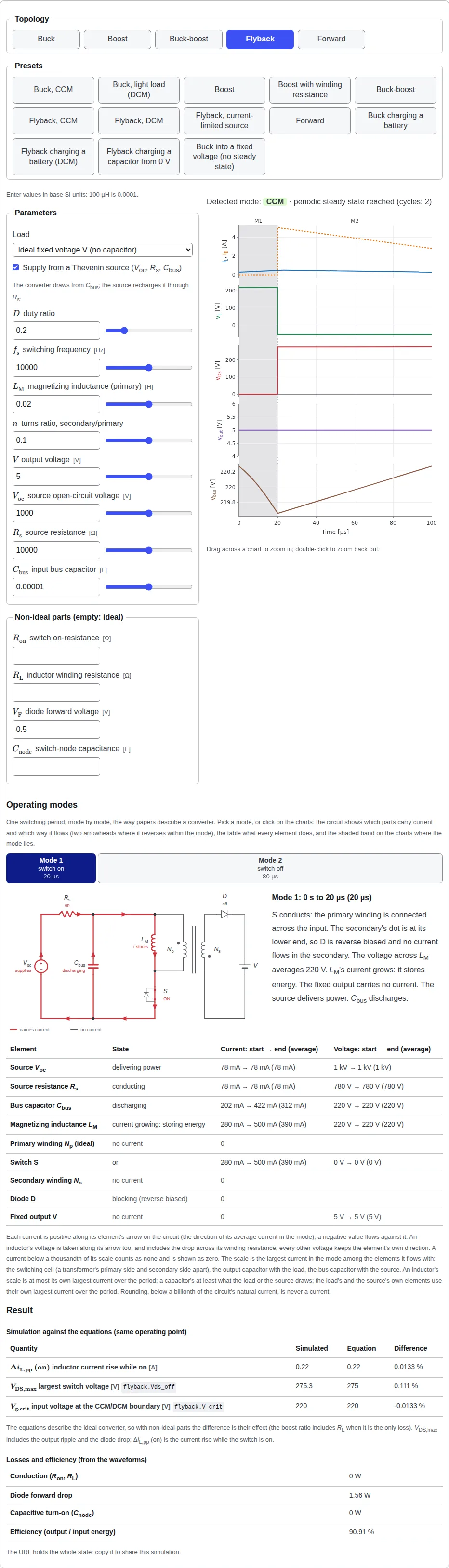
The numbers in the examples, presets and exercises on this site are synthetic: round teaching values, not data from any real design.